In my previous article (CODE Magazine, July/August 2016) on the Internet of Things (IoT), I mentioned the two components of IoT: Data Collection and Data Analysis. In that article, you learned how the Python language was used to program your Raspberry Pi for data collection, talking to all the different sensors and at the same time allowing you to use it to write server-side apps for communicating with third-party servers (such as for push notifications). In this article, I'm going to turn my attention to the second component of IoT: Data Analysis.
In recent years, you've often heard the term Data Science. According to Wikipedia, Data Science is "an interdisciplinary field about processes and systems to extract knowledge or insights from data in various forms, either structured or unstructured, which is a continuation of some of the data analysis fields, such as statistics, data mining, and predictive analytics, similar to Knowledge Discovery in Databases (KDD)". In simple terms, Data Science involves using tools to derive meaning from a huge pool of data, allowing you to draw conclusions about the past or predict the future.
In simple terms, Data Science involves using tools to derive meanings from a huge pool of data, allowing you to make conclusions about the past or predict the future.
Data Science is a big subject and just one article doesn't do it justice. But you need to start somewhere. In this article, I'll start by introducing you to some of the tools commonly used in Data Science. You'll see that because Python is such a widely used language, and coupled with an active community of Python libraries developers, it's no coincidence that Python is a favorite language among data scientists.
A Quick Introduction to Python
Before I get to the heart of Data Science using Python, it's important to ground yourself in the basics of one of the key data types in Python: list. A lot of operations that you can perform on a list apply to the other data types that you'll see later in this article, so now's a good time to take a look.
In Python, a list is a collection of values:
lst = [4,"Hello", 3.14, True]
print(lst)      # [4, 'Hello', 3.14, True]
As you can see in the output above, the items in a list need not be of the same type – in that snippet, there's a mixture of integer, string, double, and Boolean values. To access the items in a list, you use an index (starting at 0):
print(lst[0])   # 4
print(lst[1])   # Hello
print(lst[2])   # 3.14
print(lst[3])   # True
Slicing Lists in Python
When you're dealing with lists, you usually want to extract a group of items from them, not just a single one. For this purpose, Python has this concept known as slicing.
Slicing extracts one or more elements from a list.
Slicing in Python has the following syntax:
list[start:end:step]
As you can see in that snippet, start is the index of the starting item, end is the index of the last item (which is not included in the answer), and step is the number of items to advance. If any of those parameters is omitted, the following defaults are assumed:
- If
startis omitted, it's assumed to be 0. - If
endis omitted, it's assumed to be the length of the list. - If
stepis omitted, it's assumed to be 1.
Let's take a look at some examples. The following statement prints out the items from index 0 to 1 (remember that the item at index 2 isn't returned in the answer):
print(lst[0:2]) # [4, 'Hello']
An easy way to understand the above syntax is to interpret it this way: get (2-0) items from the list starting from index 0.
The following snippet prints out the items from index 1 to 1 and only one item is returned:
print(lst[1:2]) # ['Hello']
If you use this the way I showed you in the previous example to interpret the syntax, that's: get (2-1) items from the list starting from index 1.
The following statement prints out all the items starting from index 1:
print(lst[1:]) # ['Hello', 3.14, True]
Notice that in this case, the end isn't specified. Its value defaults to the length of the list, which is four items. So the above is essentially the same as:
print(lst[1:4])
The following statement prints the first three elements:
print(lst[:3]) # [4, 'Hello', 3.14]
In this case, the start isn't specified so it defaults to 0, which is essentially the same as:
print(lst[0:3])
The following statement prints all items in the list except the last two:
print(lst[:-2]) # [4, 'Hello']
The following statement prints the last two items:
print(lst[-2:]) # [3.14, True]
The following statement reverses all the items in the list:
print(lst[::-1]) # [True, 3.14, 'Hello', 4]
The following statement prints all of the items starting from index 0 to 4, and a step of 2, which means that it prints items at index 0 and 2:
print(lst[0:4:2]) # [4, 3.14]
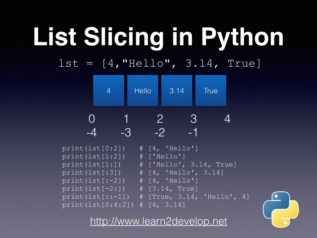
If you have difficulty remembering how slicing works in Python, you can use the method shown in Figure 1. Just imagine the index to be sandwiched between the elements and it will be very easy for you to understand how slicing works.
Extending Python's List DataType using NumPy
The key problem with the Python's list data type is its efficiency. A list allows you to have non-uniform type items; each item in the list is stored in a memory location, with the list containing an array of pointers to each of these locations. A Python list requires:
- At least 4 bytes per pointer
- At least 16 bytes for the smallest Python object: 4 bytes for the pointer, 4 bytes for the reference count, and 4 for the value. These round up to 16 bytes.
Because of the way the Python list is implemented, accessing items in a large list is computationally expensive. To solve this problem, you can use NumPy. NumPy is an extension to the Python programming language, adding support for large, multi-dimensional arrays and matrices, along with a large library of high-level mathematical functions to operate on these arrays.
NumPy Array Basics
In NumPy, an array is of type ndarray (n-dimensional array). A NumPy array is an array of homogeneous values (all of the same type), and all items occupy a contiguous block of memory.
To use NumPy, you first need to import the numpy package:
import numpy as np
Array operations are very similar to that of the Python list. For example, the following code snippet creates a Python list and then converts it to a NumPy array:
l1 = [1,2,3,4,5]
array1 = np.array(l1) # rank 1 array
In this case, array1 is known as a rank 1 (one dimensional) array. You can print out the array as usual using the print() function:
print (array1) # [1 2 3 4 5]
You can print out the shape of the array using the shape property:
print (array1.shape) # (5,)
The shape property returns a tuple containing the dimension of the array. In the above example, array1 is a 1-dimensional array of five items.
Just like Python list, you can access items in the NumPy array using indexing as well as slicing:
print (array1.shape)   # (5,)
print (array1[0])      # 1
print (array1[1])      # 2
print (array1[1:3])    # [2 3]
print (array1[:-2])    # [1 2 3]
print (array1[3:])     # [4 5]
You can also pass in a list containing the index of the items you want to extract to the array:
print (array1[[2,3]]) # [3,4]
The following code snippet shows how you can create a two-dimensional array:
l2 = [6,7,8,9,0]
array2 = np.array([l1,l2])  # rank 2 array
print (array2)
'''
[[1 2 3 4 5]
 [6 7 8 9 0]]
'''
print (array2.shape)        # (2,5) - 2 rows and
                            # 5 columns
print (array2[0,0])         # 1
print (array2[0,1])         # 2
print (array2[1,0])         # 6
Creating and Initializing Arrays using NumPy
NumPy contains a number of helper functions that make it easy to initialize arrays with some default values. For example, if you want to create an array containing all zeroes, you can use the zeros() function with a number indicating the size of the array:
a1 = np.zeros(2)   # array of rank 1 with all 0s
print a1.shape     # (2,)
print a1[0]        # 0.0
print a1[1]        # 0.0
If you want to create a rank 2 array, simply pass in a tuple:
a2 = np.zeros((2,3)) # array of rank 2 with all 0s;
                     # 2 rows and 3 columns
print a2.shape       # (2,3)
print a2
'''
 [[ 0.  0.  0.]
  [ 0.  0.  0.]]
'''
To initialize the array to some other values other than zeroes, use the full() function:
a3 = np.full((2,3), 8)     # array of rank 2
                           # with all 8s
print a3
'''
[[ 8.  8.  8.]
 [ 8.  8.  8.]]
'''
In linear algebra, you often need to deal with an identity matrix, and you can create this in NumPy easily with the eye() function:
a4 = np.eye(4)             # 4x4 identity matrix
print a4
'''
[[ 1.  0.  0.  0.]
 [ 0.  1.  0.  0.]
 [ 0.  0.  1.  0.]
 [ 0.  0.  0.  1.]]
'''
And if you need to populate an array with some random values, you can use the random.random() function to generate random values between 0.0 and 1.0:
a5 = np.random.random((2,4)) # populate a rank 2
                             # array (2 rows
                             # 4 columns) with
                             # random values
print a5
'''
[[ 0.21135397  0.39570425  0.25548923  0.05606163]
 [ 0.14495175  0.19093966  0.29366716  0.61189549]]
'''
Finally, you can create a range of values from 0 to n-1 using the arange() function:
a6 = np.arange(10)  # creates a range from 0 to 9
print a6            # [0 1 2 3 4 5 6 7 8 9]
Boolean Array Indexing
One of the many useful features of the NumPy array is its support for array boolean indexing. Consider the following example: You have a list of numbers and you need to retrieve all of the even numbers from the list. Using Python's list, you need to iterate through all items in the list and perform a check individually. Using NumPy array, however, things are much easier. Look at the following example:
nums = np.array([23,45,78,89,23,11,22])
You first specify the condition, testing for even numbers, and then assign it to a variable:
even_nums = nums % 2 == 0
The even_nums variable is now a NumPy array, containing a collection of Boolean values. If you print it out, you'll see just that:
print (even_nums)
'''
[False False  True False False False  True]
'''
The True values indicate that the particular item is an even number. Using this Boolean array, you can now use it as an index to the numbers array:
print (nums[even_nums])
'''
[78 22]
'''
The above statements could be written succinctly like this:
print (nums[nums % 2 == 0])
The array boolean indexing feature makes it extremely useful to manipulate a large amount of data without worrying about the underlying implementation. Here's another example:
prices = np.array([45,23,56,89,12,48])
reasonable = (prices > 20) & (prices < 50)
print prices[reasonable]
'''
[45 23 48]
'''
Array Math
Another area where the NumPy array excels is in array math. Consider the following rank-2 arrays:
x1 = np.array([[1,2,3],[4,5,6]])
y1 = np.array([[7,8,9],[2,3,4]])
You can add each of the two arrays' items by using the + operator on the two arrays:
print x1 + y1
'''
[[ 8 10 12]
 [ 6  8 10]]
'''
Alternatively, you can also use the add() function to add the two arrays:
np.add(x1,y1)
Likewise, you can subtract, multiply, and divide arrays directly:
print x1 - y1     # same as np.subtract(x1,y1)
'''
[[-6 -6 -6]
 [ 2  2  2]]
'''
print x1 * y1     # same as np.multiply(x1,y1)
'''
[[ 7 16 27]
 [ 8 15 24]]
'''
print x1 / y1     # same as np.divide(x1,y1)
'''
[[0 0 0]
 [2 1 1]]
'''
Very often, you need to generate the cumulative sum of a series of numbers. NumPy's array makes it really easy. Suppose you have the following array:
a = np.array([(1,2,3), (4,5,6), (7,8,9)])
print (a)
'''
[[1 2 3]
 [4 5 6]
 [7 8 9]]
'''
To generate the cumulative sum of all the numbers in the array, use the cumsum() function:
print (a.cumsum())   # prints the cumulative sum
                     # of all the elements in
                     # the array
'''
[ 1  3  6 10 15 21 28 36 45]
'''
Note that the result is returned as a rank-1 array.
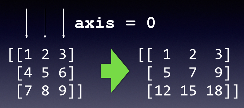
To generate a cumulative sum over the rows for each of the columns, specify the axis parameter with a value of 0:
print (a.cumsum(axis=0))  # sum over rows for
                          # each of the 3
                          # columns
'''
[[ 1  2  3]
 [ 5  7  9]
 [12 15 18]]
'''
Figure 2 shows how the cumulative sums are generated when the axis parameter is set to 0.
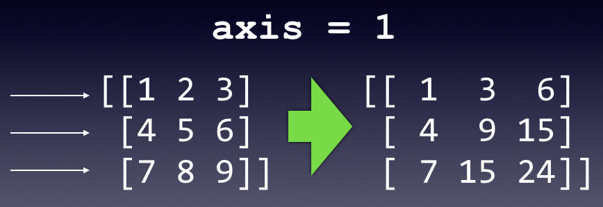
To generate a cumulative sum over the columns for each of the rows, specify the axis parameter with a value of 1:
print (a.cumsum(axis=1))  # sum over columns for
                          # each of the 3 rows
'''
[[ 1  3  6]
 [ 4  9 15]
 [ 7 15 24]]
'''
Figure 3 shows how the cumulative sums are generated when the axis parameter is set to 1.
Visualizing Data using Matplotlib
As the saying goes, a picture's worth a thousand words. With huge amount of data, there's no better way to understand the data than to visualize it graphically. A popular charting application for Python is the matplotlib library. The matplotlib library is a Python 2D plotting library, which produces publication quality figures. What's more, a lot of Python libraries, like NumPy and Pandas (discussed in the next section), have inherent support for it, making plotting very accessible.
Consider the following code snippet:
%matplotlib inline
import matplotlib.pyplot as plt

plt.plot(
    [1,2,3,4,5,6,7,8,9,10],
    [2,4.5,1,2,3.5,2,1,2,3,2]
)
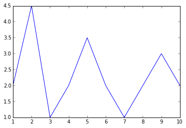
First, the %matplotlib inline statement tells Jupyter Notebook to display the matplotlib chart inline, rather than in a separate window. To plot charts, use the matplotlib library's pyplot module and import it as plt (by convention). The plot() function displays a default line chart with the first argument (a Python list) on the x-axis and the second argument (also a Python list) as the y-axis. The result is as shown in Figure 4.
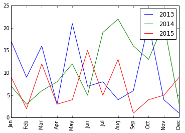
Although you can plot a matplotlib chart using Python lists, you can often plot it using NumPy arrays. Consider another example, where you've recorded the number of rainy days per month for the past three years. You want to plot this data on the same chart and do a visual comparison.
Listing 1 is the code to plot three line charts in a single figure, showing the number of rainy days per month for the past three years.
Listing 1: Plotting the number of rainy days per month for the past three years
%matplotlib inline
import numpy as np
import matplotlib.pyplot as plt

year_2013 = [17,9,16,3,21,7,8,4,6,21,4,1]
year_2014 = [7,3,6,8,12,5,19,22,16,13, 21,3]
year_2015 = [9,2,12,3,4,15,5,13,1,4,5,9]

rainy_days = np.array([year_2013,year_2014,year_2015])

labels = ['Jan','Feb','Mar','Apr','May','Jun',
          'Jul','Aug','Sep','Oct','Nov','Dec']

plt.xticks(range(len(year_2013)), labels, rotation='vertical')

year = 2013
for month in rainy_days:
    plt.plot(month, label=year) # plot the rainy days for each year
    year += 1

plt.legend()                    # show the legend
plt.show()
The xticks() function sets the locations and labels of the ticks on the x-axis. In this example, I've set it to display the shorthand for each month and make them display vertically (see Figure 5).
Very often, your data is stored in files, such as Excel or CSV files. NumPy makes it easy to load and use data from files. Suppose there's a CSV file named results.csv containing the grade results of a student for 10 semesters:
1,2
2,4.5
3,1
4,2
5,3.5
6,2
7,1
8,2
9,3
10,2
You can load the file into a NumPy array as follows:
import numpy as np

semester,grade = np.loadtxt("results.csv", unpack=True,
                            delimiter=",")
The loadtxt() function loads the data from the specified text file. The unpack argument indicates whether the returned array is unpacked as individual arrays for each field, and the delimiter argument specifies the delimiter used to separate the various fields in the text file. The semester variable is now an array containing the values from 1 to 10, and the grade variable is an array containing the grades (2,4.5, … ,2).
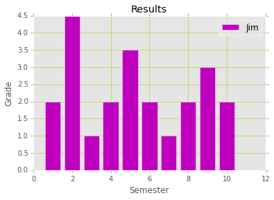
Listing 2 shows the code to plot a bar chart using the data loaded from the CSV file.
Listing 2: Plotting a bar chart from data loaded from a CSV file
from matplotlib import pyplot as plt
from matplotlib import style
import numpy as np

style.use("ggplot")

semester,grade = np.loadtxt("results.csv", unpack=True,
                            delimiter=",")

plt.bar(
    semester,
    grade,
    label="Jim",
    color = "m",
    align= "center"
)

plt.title("Results")       # sets the title
plt.xlabel("Semester")     # sets the label for x-axis
plt.ylabel("Grade")        # sets the label for y-axis

plt.legend()               # shows the legend
plt.grid(True, color="y")  # shows and sets the grid color to yellow
The generated chart is as shown in Figure 6.
Manipulating Data and Performing Data using Pandas
Although NumPy arrays are a much improved version over Python's list, it's insufficient to meet the needs of data science. In the real world, data is often presented in table formats. For example, consider the content of the CSV file shown in Listing 3.
Listing 3: The readings of a person's blood glucose readings stored in a CSV file
,DateTime,mmol/L
0,2016-06-01 08:00:00,6.1
1,2016-06-01 12:00:00,6.5
2,2016-06-01 18:00:00,6.7
3,2016-06-02 08:00:00,5.0
4,2016-06-02 12:00:00,4.9
5,2016-06-02 18:00:00,5.5
6,2016-06-03 08:00:00,5.6
7,2016-06-03 12:00:00,7.1
8,2016-06-03 18:00:00,5.9
9,2016-06-04 09:00:00,6.6
10,2016-06-04 11:00:00,4.1
11,2016-06-04 17:00:00,5.9
12,2016-06-05 08:00:00,7.6
13,2016-06-05 12:00:00,5.1
14,2016-06-05 18:00:00,6.9
15,2016-06-06 08:00:00,5.0
16,2016-06-06 12:00:00,6.1
17,2016-06-06 18:00:00,4.9
18,2016-06-07 08:00:00,6.6
19,2016-06-07 12:00:00,4.1
20,2016-06-07 18:00:00,6.9
21,2016-06-08 08:00:00,5.6
22,2016-06-08 12:00:00,8.1
23,2016-06-08 18:00:00,10.9
24,2016-06-09 08:00:00,5.2
25,2016-06-09 12:00:00,7.1
26,2016-06-09 18:00:00,4.9
The CSV file contains rows of data divided into three columns: index, date and time of recording, and blood glucose readings in mmol/L.
To be able to deal with data stored as tables, you need a new data type that's more suited to deal with it: That means that you want pandas. Pandas is a Python package providing fast, flexible, and expressive data structures designed to make working with “relational” or “labeled” data both easy and intuitive.
Although Python supports lists and dictionaries for manipulating structured data, it's not well-suited for manipulating numerical tables, such as the one stored in the CSV file.
Pandas supports two key data structures: Series and DataFrame. Let's take a closer look at these two data structures before I come back to look at how to use pandas to manipulate the blood glucose readings data.
Series
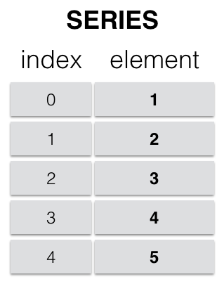
A Series is a one-dimensional NumPy-like array, with each element having an index (0, 1, 2,… by default); a Series behaves like a dictionary, with an index. Figure 7 shows the structure of a Series in pandas.
The following code snippet shows how a Series can be created in pandas:
import pandas as pd

series = pd.Series([1,2,3,4,5])
print series
'''
0    1
1    2
2    3
3    4
4    5
dtype: int64
'''
Like NumPy, you need to import the pandas package before using it. The Series() function creates a pandas series from a list of items.
One good use of Series is for generating date ranges.
One good use of Series is for generating date ranges. Consider the following example:
import pandas as pd

dates1 = pd.date_range('20160525', periods=12)
print dates1
'''
DatetimeIndex(['2016-05-25', '2016-05-26',
               '2016-05-27', '2016-05-28',
               '2016-05-29', '2016-05-30',
               '2016-05-31', '2016-06-01',
               '2016-06-02', '2016-06-03',
               '2016-06-04', '2016-06-05'],
              dtype='datetime64[ns]', freq='D')
'''
The date_range() function creates a series representing a series of dates. The periods parameter allows you to specify the date intervals. For example, in this case, 12 means 12 days starting with the specified date, which is 25 May 2016.
You can also specify the frequency using the freq parameter:
dates2 = pd.date_range('2016-05-01', periods=12,
                       freq='M')
print dates2
'''
DatetimeIndex(['2016-05-31', '2016-06-30',
               '2016-07-31', '2016-08-31',
               '2016-09-30', '2016-10-31',
               '2016-11-30', '2016-12-31',
               '2017-01-31', '2017-02-28',
               '2017-03-31', '2017-04-30'],
              dtype='datetime64[ns]', freq='M')
'''
The default frequency is in days, but if you specified M for freq, the frequency is changed to monthly. You can even change the frequency to hourly:
dates3 = pd.date_range('2016/05/17 09:00:00',
                       periods=8,
                       freq='H')
print dates3
'''
DatetimeIndex(['2016-05-17 09:00:00',
               '2016-05-17 10:00:00',
               '2016-05-17 11:00:00',
               '2016-05-17 12:00:00',
               '2016-05-17 13:00:00',
               '2016-05-17 14:00:00',
               '2016-05-17 15:00:00',
               '2016-05-17 16:00:00'],
              dtype='datetime64[ns]', freq='H')
'''
Observe that in each of the above examples, the date_range() function is smart enough to detect the date format passed in (the first one uses YYYYMMDD, and the second one uses YYYY-MM-DD, and the third one uses YYYY/MM/DD).
DataFrame
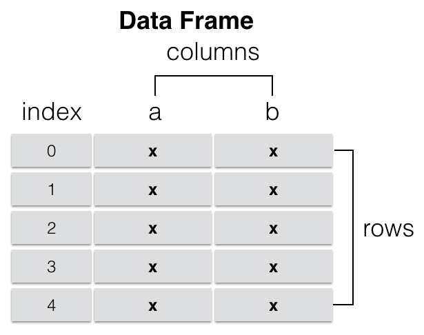
A DataFrame is a two-dimensional NumPy-like array. Think of it as a table. Figure 8 shows the structure of a DataFrame in pandas.
The following code snippet shows how a DataFrame can be created in pandas:
import pandas as pd
import numpy as np

data_frame = pd.DataFrame(np.random.randn(10,4),
                          columns=list('ABCD'))
print data_frame
First, you use the random.randn() function to generate an array of the specified shape (10 rows and four columns; in this example) filled with random floating-point numbers sampled from a univariate “normal” (Gaussian) distribution of mean 0 and variance 1. The columns parameter specifies a list containing the column headers. Here, you're creating a list from a string ('ABCD'). The DataFrame created looks like this:
'''
          A         B         C         D
0  1.269108 -0.496408 -0.162528  0.432953
1 -0.895156 -0.014969  0.383383  1.902658
2 -1.292945  0.656012  0.376739  0.875683
3  0.456998  0.863970  1.155423  0.587762
4 -0.630788  0.006764  0.734363  0.975344
5  0.277726  0.947913 -0.838228 -0.318126
6 -2.095660  0.757282 -0.917780 -0.345179
7 -1.399808 -2.210822 -2.009842 -1.449238
8 -1.801125  0.463970 -0.817592  1.147401
9 -0.938238  0.028543 -0.774980 -0.195423
'''
Notice that the index is automatically created for the DataFrame. If you wish, you can change the index to something else, such as date and time. For example, the following code snippet shows using a Series as the index for the DataFrame:
days = pd.date_range('20150525', periods=10)
data_frame = pd.DataFrame(np.random.randn(10,4),
                          index=days,
                          columns=list('ABCD'))
print data_frame
The index parameter is assigned a Series (days), which is generated by the date_range() function. The DataFrame now looks like this:
'''
                   A         B         C         D
2015-05-25 -0.181824 -0.522341 -0.629486 -0.098926
2015-05-26 -0.786451  0.270572 -0.007755  0.407279
2015-05-27 -1.801745 -0.627653  0.017884 -0.294941
2015-05-28 -0.199777 -0.343533 -0.847143  0.230196
2015-05-29 -0.470902 -1.882163  1.589637  0.041875
2015-05-30  0.223365 -0.367830  0.901914 -1.574907
2015-05-31 -0.701686  2.185077 -0.787870 -1.014857
2015-06-01  2.078889  0.467649  0.462715  0.731940
2015-06-02 -0.739564  0.055060 -0.414679  1.229497
2015-06-03  1.086807  0.134102 -1.114484 -0.277467
'''
Selecting Data From DataFrames
There are many ways to select data from a DataFrame. Let me highlight a few examples. First, to display a specific column, pass in the column header as the index, like this:
print data_frame['A'] # prints column A
This prints out the index as well as all of column A:
'''
2015-05-25    0.400942
2015-05-26    0.553610
2015-05-27   -1.772219
2015-05-28    0.298267
2015-05-29   -0.079830
2015-05-30    0.619363
2015-05-31   -0.217129
2015-06-01   -0.111042
2015-06-02    1.080578
2015-06-03    1.937649
'''
Because the index of the data_frame is a date range, you can perform slicing, like this:
# prints rows with index from 2015-05-25 to 2015-05-28
print data_frame['2015-05-25':'2015-05-28']
The result is as follows:
'''
                   A         B         C         D
2015-05-25  0.400942  0.734476 -0.900102 -0.148904
2015-05-26  0.553610  1.729898  1.248708  0.353235
2015-05-27 -1.772219 -2.182172 -0.439986 -1.672310
2015-05-28  0.298267  1.049802 -2.093472  1.330577
'''
You can also perform slicing using row numbers:
print data_frame[2:5]     # prints row 3 through
                          # row 5
The above statement prints all the rows from index 2 to 5 (not included in the result), which means from row 3 to row 5:
'''
                   A         B         C         D
2015-05-27 -1.772219 -2.182172 -0.439986 -1.672310
2015-05-28  0.298267  1.049802 -2.093472  1.330577
2015-05-29 -0.079830  1.169019  0.047177 -0.599912
'''
Very often when plotting charts, you need to flip the columns and rows of the DataFrame, and this can be accomplished using the T property:
print data_frame.T
The T property transposes (interchanges) the index and columns of the DataFrame:
'''
  2015-05-25  2015-05-26  2015-05-27  2015-05-28
2015-05-29  2015-05-30  \
A   0.575812   -0.401051   -1.767028    1.148867
-1.013309   -0.232075
B  -0.994374   -0.225347   -0.683786    1.600078
0.655725    0.210781
C  -0.641241    1.003547    0.308813    1.066649
-0.181266    0.140533
D  -0.384547    0.256077   -0.980992    0.647792
0.151229    0.260636
  2015-05-31  2015-06-01  2015-06-02  2015-06-03
A  -0.892355   -0.178719   -0.174579   -0.364807
B  -1.073592    0.985476   -1.347515   -0.735336
C  -0.260684   -0.706353   -0.872690    1.385756
D   1.456331   -1.800571    0.416017   -0.392111
'''
Plotting in Pandas
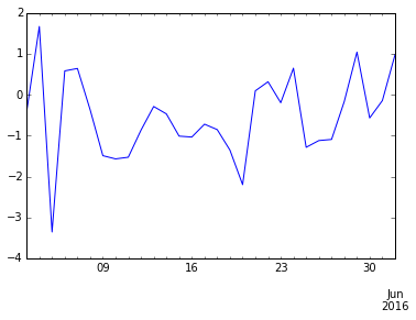
Like NumPy arrays, you can directly plot using matplotlib from a Series or DataFrame. The following code snippet plots a line chart from a panda Series (see Figure 9 for the chart):
%matplotlib inline
import pandas as pd
import numpy as np

series = pd.Series(np.random.randn(30),
                 pd.date_range(end='2016-06-01',
                 periods=30))
series.plot()
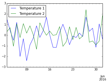
The following code snippet plots a line chart from a Panda DataFrame (see Figure 10 for the chart):
%matplotlib inline
import pandas as pd
import numpy as np

series = pd.Series(np.random.randn(30),
                pd.date_range(end='2016-06-01',
                periods=30))

data_frame = pd.DataFrame(np.random.randn(30,2),
                       index=series.index,
                       columns=
                       ['Temperature 1',
                        'Temperature 2'])
data_frame.plot()
The
plot()function on Series and DataFrame is just a simple wrapper aroundpyplot.plot().
A Sample Case Study: Visualizing Blood Glucose Readings Data
Healthcare is one area that receives a lot of consideration from technology. One particular disease, diabetes, garners a lot of attention. According to the World Health Organization (WHO), the number of people with diabetes has risen from 108 million in 1980 to 422 million in 2014. The care and prevention of diabetes is obviously of paramount importance. Diabetics need to regularly measure the amount of sugar in their blood.
For this case study, I'm going to show you how to visualize the data collected by a diabetic so that he can see at a glance how well he is keeping diabetes under control.
Data Source
For this case study, I'm assuming that you have a CSV file named readings.csv, which was shown earlier in Listing 3. The CSV file contains rows of data that are divided into three columns: index, date and time, and blood glucose readings in mmol/L.
Reading the Data in Python
To read the data from the CSV file into your Python app, use the following code snippet:
import pandas as pd

data_frame = pd.read_csv('readings.csv',
                         index_col=0,
                         parse_dates=[1])
print data_frame
You first import the pandas module, then you use the read_csv() function to read the data from the CSV file to create a DataFrame. The index_col parameter specifies which column in the CSV file will be used as the index (column 0 in this case) and the parse_dates parameter specifies the column that should be parsed as a datetime object (column 1 in this case).
When you print out the dataframe, you should see the following:
              DateTime  mmol/L
0  2016-06-01 08:00:00     6.1
1  2016-06-01 12:00:00     6.5
2  2016-06-01 18:00:00     6.7
3  2016-06-02 08:00:00     5.0
4  2016-06-02 12:00:00     4.9
5  2016-06-02 18:00:00     5.5
6  2016-06-03 08:00:00     5.6
7  2016-06-03 12:00:00     7.1
8  2016-06-03 18:00:00     5.9
9  2016-06-04 09:00:00     6.6
10 2016-06-04 11:00:00     4.1
11 2016-06-04 17:00:00     5.9
12 2016-06-05 08:00:00     7.6
13 2016-06-05 12:00:00     5.1
14 2016-06-05 18:00:00     6.9
15 2016-06-06 08:00:00     5.0
16 2016-06-06 12:00:00     6.1
17 2016-06-06 18:00:00     4.9
18 2016-06-07 08:00:00     6.6
19 2016-06-07 12:00:00     4.1
20 2016-06-07 18:00:00     6.9
21 2016-06-08 08:00:00     5.6
22 2016-06-08 12:00:00     8.1
23 2016-06-08 18:00:00    10.9
24 2016-06-09 08:00:00     5.2
25 2016-06-09 12:00:00     7.1
26 2016-06-09 18:00:00     4.9
Visualizing the Data
Let's now try to visualize the data by displaying a chart. Add the indicated statements to the existing Python script:
%matplotlib inline                          # Add this line
import pandas as pd
data_frame = pd.read_csv('readings.csv',
                         index_col=0,
                         parse_dates=[1])
print data_frame
data_frame.plot(x='DateTime', y='mmol/L')   # Add this line
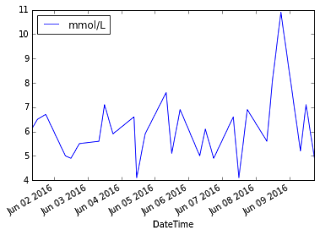
The x parameter specifies the column to use for the x-axis and the y parameter specifies the column to use for the y-axis. This displays the chart as shown in Figure 11.
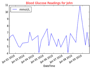
You can add a title to the chart by importing the matplotlib.pyplot module and using the title() function:
%matplotlib inline
import pandas as pd
import matplotlib.pyplot as plt              # Add this line

data_frame = pd.read_csv('readings.csv',
                         index_col=0,
                         parse_dates=[1])
print data_frame
data_frame.plot(x='DateTime', y='mmol/L')
plt.title('Blood Glucose Readings for John',  # Add this line
          color='Red')
A title is now displayed for the chart (see Figure 12).
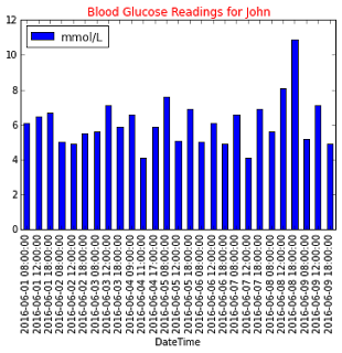
By default, matplotlib displays a line chart. You can change the chart type by using the kind parameter:
data_frame.plot(kind='bar', x='DateTime', y='mmol/L') # kind='bar'
The chart is now changed to a bar chart (see Figure 13).
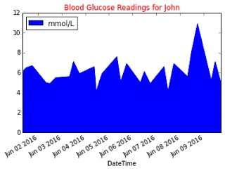
Besides displaying as a bar chart, you can also display an area chart:
data_frame.plot(kind='area', x='DateTime', y='mmol/L') # kind='area'
The chart is now displayed as an area chart (see Figure 14).
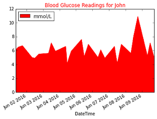
You can also set the color for the area chart by using the color parameter:
data_frame.plot(kind='area', x='DateTime', y='mmol/L',
                color='r')                                # color='r'
The area is now in red (see Figure 15).
Summary
In this article, I've touched on the foundation of Data Science, using Python and its companion libraries, NumPy, pandas, and matplotlib, and you've learned to manipulate data and present them in a visual manner. In a future article, I'll delve deeper into the world of Data Science.


