In my previous article (“Getting Started with Machine Learning Using Microsoft Azure ML Studio”, http://www.codemag.com/article/1709071), I explained the concepts behind machine learning and got you started using the Microsoft Azure Machine Learning Studio (MAML). For beginners, the MAML is a really good way to dabble with machine learning without possessing the mathematical prerequisites that are usually required of a data scientist. However, to really implement machine learning, you need to move beyond MAML and be able to implement your learning models programmatically. This has the advantage of fine-tuning the models to your needs, and, at the same time, affording you the flexibility to deploy the models in whatever manner you want.
One of the languages that's most popular with data scientists is Python. With its vast amount of third-party library support, Python is well-suited for implementing machine learning. In this article, I'll build a couple of models using Python and its accompanying library Scikit-learn. Although Python is popular among data scientists, another language remains popular among statisticians: R. I don't have the luxury of space to delve into R programming in this article, but I'll provide the solution for the Titanic problem in both Python and R so that enthusiasts can devour them over the weekends.
Introduction to Scikit-learn
In one of my earlier articles on Data Science (Introduction to Data Science using Python), you learned how to use Python together with libraries such as NumPy and Pandas to perform number crunching, data visualization, and analysis. For machine learning, you can also use these libraries to build learning models. However, doing so requires that you have a strong appreciation of the mathematical foundation for the various machine learning algorithms. This isn't a trivial matter. Instead of implementing the various machine-learning algorithms manually, fortunately, someone else has already done the hard work for you.
Scikit-learn is a Python library that implements the various types of machine learning algorithms, such as classification, regression, clustering, decision tree, and more. Using Scikit-learn, implementing machine learning is now simply a matter of supplying the appropriate data to a function so that you can fit and train the model.
Getting Datasets
Often, one of the challenges in machine learning is obtaining sample datasets for experimentation. Fortunately, Scikit-learn comes with a few standard sample datasets, which makes learning machine learning easy.
To load the sample datasets, import the datasets module and load the desired dataset. For example, the following code snippets load the Iris dataset:
from sklearn import datasets
iris = datasets.load_iris()
print(iris)         # raw data of type Bunch
The dataset loaded is a Bunch object, which is a Python dictionary that provides attribute-style access. You can use the DESCR property to obtain a description of the dataset:
print(iris.DESCR)
More importantly, you can obtain the features of the dataset using the data property:
print(iris.data) # Features
The above statement prints the following:
[[ 5.1  3.5  1.4  0.2]
 [ 4.9  3.   1.4  0.2]
...
 [ 6.2  3.4  5.4  2.3]
 [ 5.9  3.   5.1  1.8]]
You can also use the feature_names property to print the names of the features:
print(iris.feature_names) # Feature Names
The above statement prints the following:
['sepal length (cm)', 'sepal width (cm)', 'petal length (cm)', 'petal width (cm)']
This means that the dataset contains four columns: sepal length, sepal width, petal length, and petal width. To print the label of the dataset, use the target property. For the label names, use the target_names property:
print(iris.target)             # Labels
print(iris.target_names)       # Label names
The above prints out the following:
[0 0 0 0 0 0 0 0 0 0 0 0 0 0 0 0 0 0 0 ...
2 2 2 2 2 2 2 2]
['setosa' 'versicolor' 'virginica']
Note that not all sample datasets support the feature_names and target_names properties.
Figure 1 summarizes how the dataset looks:

Often, it's useful to convert the data to a Pandas DataFrame so that you can manipulate it easily:
import pandas as pd
df = pd.DataFrame(iris.data)
            # convert features
            # to dataframe in Pandas
print(df.head())
The above statements print out the following:
0    1    2    3
0  5.1  3.5  1.4  0.2
1  4.9  3.0  1.4  0.2
2  4.7  3.2  1.3  0.2
3  4.6  3.1  1.5  0.2
4  5.0  3.6  1.4  0.2
Besides of the Iris dataset, you can also load some interesting datasets, such as the following:
# data on breast cancer
breast_cancer = datasets.load_breast_cancer()

# data on diabetes
diabetes = datasets.load_diabetes()

# dataset of 1797 8x8 images of hand-written digits
digits = datasets.load_digits()
Solving Regression Problems Using Linear Regression
The easiest way to get started is with Linear Regression. Linear Regression is a linear approach for modeling the relationship between a scalar dependent variable Y and one or more explanatory variables (or independent variables). For example, let's say that you have a set of data consisting of the heights of a group of people and their corresponding weights:
%matplotlib inline
import matplotlib.pyplot as plt

# represents the heights of a group of people
heights = [[1.6], [1.65], [1.7], [1.73], [1.8]]

# represents the weights of a group of people
weights = [[60], [65], [72.3], [75], [80]]

plt.title('Weights plotted against heights')
plt.xlabel('Heights in metres')
plt.ylabel('Weights in kilograms')

plt.plot(heights, weights, 'k.')

# axis range for x and y
plt.axis([1.5, 1.85, 50, 90])
plt.grid(True)
When you plot a chart of weights against heights, you'll see the figure shown in Figure 2.
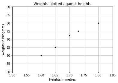
From the chart, you can see that there's a positive co-relation between the weights and heights for that group of people. You could draw a straight line through the points and use that to predict the weight of another person based on height.
Using the LinearRegression Class for Fitting the Model
So how do you draw the straight line that cuts though all the points? It turns out that the Scikit-learn library has a LinearRegression class that helps you to do just that. All you need to do is to create an instance of this class and use the heights and weights lists to create a linear regression model using the fit() function, like this:
from sklearn.linear_model
import LinearRegression

# Create and fit the model
model = LinearRegression()
model.fit(heights, weights)
Once you've fitted the model, you can start to make predictions using the predict() function, like this:
# make prediction
weight = model.predict([[1.75]])[0][0]
print(weight)
# 76.0387650086
Plotting the Linear Regression Line
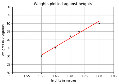
It would be useful to visualize the linear regression line that's been created by the LinearRegression class. Let's do this by first plotting the original data points and then sending the heights list to the model to predict the weights. Then plot the series of forecasted weights to obtain the line. The following statements show how this is done:
import matplotlib.pyplot as plt

heights = [[1.6], [1.65], [1.7], [1.73], [1.8]]
weights = [[60], [65], [72.3], [75], [80]]

plt.title('Weights plotted against heights')
plt.xlabel('Heights in metres')
plt.ylabel('Weights in kilograms')

plt.plot(heights, weights, 'k.')

plt.axis([1.5, 1.85, 50, 90])
plt.grid(True)

# plot the regression line
plt.plot(heights, model.predict(heights), color='r')
Figure 3 shows the linear regression line.
Examining the Performance of the Model by Calculating the Residual Sum of Squares
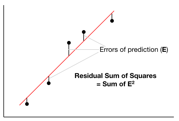
To know whether your linear regression line is well fitted to all the data points, use the Residual Sum of Squares (RSS) method. Figure 4 shows how the RSS is calculated.
The following code snippet shows how the RSS is calculated in Python:
import numpy as np

print('Residual sum of squares: %.2f' %
np.sum((weights - model.predict(heights))
** 2))

# Residual sum of squares: 5.34
The RSS should be as small as possible, with 0 indicating that the regression line fits the points exactly (rarely achievable in the real world).
Evaluating the Model Using a Test Dataset
Now that the model is fitted with the training data, you can put it to the test. You need the following test dataset:
# test data
heights_test = [[1.58], [1.62], [1.69], [1.76], [1.82]]
weights_test = [[58], [63], [72], [73], [85]]
You can measure how closely the test data fits the regression line using the R-Squared method. The R-Squared method is also known as the coefficient of determination or the coefficient of multiple determinations for multiple regressions.
The formula for calculating R-Squared is shown in Figure 5.
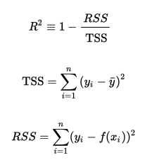
The explanation for deriving the formula for R-Squared is beyond the scope of this article, but you can visit https://en.wikipedia.org/wiki/Coefficient_of_determination for more details.
Using the formula shown for R-Squared, you can calculate R-Squared in Python using the following code snippet:
# total sum of squares
weights_test_mean = np.mean(np.ravel(weights_test))
ss_total = np.sum((np.ravel(weights_test) – weights_test_mean) ** 2)
print("ss_total: %.2f" % ss_total)

# total sum of residuals
ss_res = np.sum((np.ravel(weights_test) - np.ravel(model.predict(heights_test))) ** 2)
print("ss_res: %.2f" % ss_res)

# r_squared
r_squared = 1 - (ss_res / ss_total)
print("R-squared: %.2f" % r_squared)
The previous code snippet yields the following result:
ss_total: 430.80
ss_res: 24.62
R-squared: 0.94
Fortunately, Scikit-learn has the score() function to calculate the R-Squared automatically for you:
# using scikit-learn to calculate r-squared
print('R-squared: %.4f' % model.score(heights_test, weights_test))

# R-squared: 0.9429
A R-Squared value of 94% indicates a pretty good fit for your test data.
Solving Classification Problems Using Logistic Regression
In the previous section, you saw how linear regression works in Scikit-learn. Starting with linear regression is a good way to understand how machine learning works in Python. In this section, you're going to solve the Titanic prediction problem using another machine learning algorithm: Logistic Regression. This is the same problem that I solved in my previous article using the Microsoft Azure Machine Learning Studio (MAML). Logistic Regression is a type of classification algorithm that involves predicting the outcome of an event, such as whether a passenger will survive the Titanic disaster or not.
If you need a refresher on the Titanic problem, be sure to check out my article on machine learning in the Sep/Oct 2017 issue of CODE Magazine.
Getting the Titanic Dataset
You can get the Titanic dataset by going to https://www.kaggle.com/c/titanic/data. Once you've obtained it, you can load it into a Pandas DataFrame:
import pandas as pd
from sklearn import linear_model
from sklearn import preprocessing

# read the data
df = pd.read_csv("titanic_train.csv")
print(df.head())
It's my habit to print out the data frame at every point of the process to verify that the data is properly loaded (or cleaned, as you'll see in the next couple of sections).
Cleaning the Data
Once the data is loaded, it's time to clean the data. Among all the different fields in the Titanic dataset, there are a number of columns that aren't important in building the machine learning model. For this purpose, let's drop the columns using the following code snippets:
# drop the columns that are not useful to us
df = df.drop('PassengerId', axis=1)
# axis=1 means column

df = df.drop('Name',        axis=1)
df = df.drop('Ticket',      axis=1)
df = df.drop('Cabin',       axis=1)

# check to see if the colummns are removed
print(df.head())
You should now see the dataset shown in Listing 1.
Listing 1: The output of the dataset after dropping some columns
   Survived  Pclass     Sex   Age  SibSp  Parch     Fare Embarked
0         0       3    male  22.0      1      0   7.2500        S
1         1       1  female  38.0      1      0  71.2833        C
2         1       3  female  26.0      0      0   7.9250        S
3         1       1  female  35.0      1      0  53.1000        S
4         0       3    male  35.0      0      0   8.0500        S
Because the dataset also contains rows with missing data, let's drop them and re-index the data frame:
df = df.dropna()                # drop all rows with NaN
df = df.reset_index(drop=True)  # re-index the dataframe
print(df.head(10))
Encoding the Non-Numeric Fields
In order to perform logistic regression in Python, Scikit-learn needs the features to be encoded in numeric values. Examining the dataset, you'll see that values of Sex and Embarked are string types, and need to be encoded before you can go any further. For this purpose, you can use the LabelEncoder class to perform the conversion, like this:
# initialize label encoder
label_encoder = preprocessing.LabelEncoder()

# convert Sex and Embarked features to numeric
sex_encoded = label_encoder.fit_transform(df["Sex"])
print(sex_encoded)
# 0 = female
# 1 = male
df['Sex'] = sex_encoded

embarked_encoded = label_encoder.fit_transform(df["Embarked"])
print(embarked_encoded)
# 0 = C
# 1 = Q
# 2 = S
df['Embarked'] = embarked_encoded

print(df.head())
The last statement in the above code snippet prints out the output shown in Listing 2.
Listing 2: The values for the Sex and Embarked fields are now replaced with the encoded values
   Survived  Pclass  Sex   Age  SibSp  Parch     Fare  Embarked
0         0       3    1  22.0      1      0   7.2500         2
1         1       1    0  38.0      1      0  71.2833         0
2         1       3    0  26.0      0      0   7.9250         2
3         1       1    0  35.0      1      0  53.1000         2
4         0       3    1  35.0      0      0   8.0500         2
Note that the values for the Sex and Embarked fields are now replaced with the encoded values.
Making Fields Categorical
The next types of values that you need to take care of in the dataset is that of categorical values. Categorical types can only take on a limited, fixed number of possible values. Categorical values indicate to Scikit-learn that for this type of field, numerical operations are not possible. A good example of a categorical field is Survived, where the value can only be 0 or 1 (and not anywhere in-between).
To make a field categorical, use the Categorical class in Pandas:
# make fields categorical
df["Pclass"]   = pd.Categorical(df["Pclass"])
df["Sex"]      = pd.Categorical(df["Sex"])
df["Embarked"] = pd.Categorical(df["Embarked"])
df["Survived"] = pd.Categorical(df["Survived"])

print(df.dtypes)       # examine the datatypes for each feature
The above prints out the data types for each field, confirming that the specified four fields are converted to category:
Survived    category
Pclass      category
Sex         category
Age          float64
SibSp          int64
Parch          int64
Fare         float64
Embarked    category
dtype: object
Splitting the Dataset into Train and Test Sets
With the dataset cleaned, you're now ready to split the dataset into two distinct sets: one for training and one for testing. But before that, you need to separate the dataset into two data frames: one containing all the features and one for the label:
# we use all columns except Survived as
# features for training
features = df.drop('Survived',1)

# the label is Survived
label    = df['Survived']
In Python, to split the rows for training and testing, you can use the train_test_split() function from the model_selection module:
from sklearn.model_selection
    import train_test_split

# split the dataset into train and test sets
train_features,test_features,
train_label,test_label = train_test_split(
    features,
    label,
    test_size = 0.25, # split ratio
    random_state = 1, # Set random seed
    stratify = df["Survived"])

# Training set
print(train_features.head())
print(train_label)
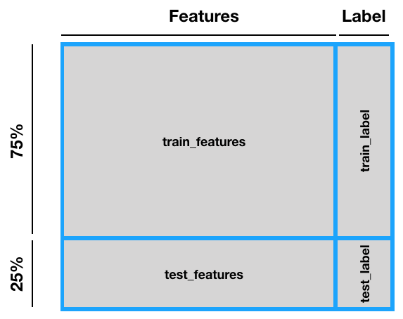
The stratify argument lets you specify a target variable to spread evenly across the train and test splits.
Figure 6 summarizes how the dataset has been split.
You can now examine the training set and its associated label:
    Pclass Sex   Age  SibSp  Parch     Fare
514      3   1  21.0      0      0   8.4333
382      3   1   9.0      5      2  46.9000
285      1   0  22.0      0      1  55.0000
142      2   1  30.0      0      0  13.0000
671      3   1  34.5      0      0   6.4375

Embarked
2
2
2
2
0

[0, 0, 1, 0, 0, ..., 0, 1, 1, 0, 0]
Length: 534
Categories (2, int64): [0, 1]
Likewise, examine the test set:
# Test set for validation
print(test_features.head())
print(test_label)
Observe that the training set has 534 rows and the test set has 178 rows, which is split in the ratio of 3:1:
    Pclass Sex   Age  SibSp  Parch     Fare
227      3   1  19.0      0      0   8.0500
318      2   1  46.0      0      0  26.0000
538      3   1  20.0      0      0   9.2250
199      1   1  37.0      1      1  52.5542
235      2   1  36.0      0      0  12.8750

Embarked
2
2
2
2
0

[1, 0, 0, 1, 0, ..., 0, 0, 1, 1, 0]
Length: 178
Categories (2, int64): [0, 1]
Training the Model
You can now go ahead and train the model. For this, use the LogisticRegression class. Train the model using the train_features against the train_label:
# initialize logistic regression model
log_regress = linear_model.LogisticRegression()
# Train the model
log_regress.fit(X = train_features ,
y = train_label)
Once the model is fitted with the data (trained), you can check its intercept and coefficients:
# Check trained model intercept
print(log_regress.intercept_)
# Check trained model coefficients
print(log_regress.coef_)
The output should look something like this:
[ 3.87427541]
[[-0.85532931 -2.30146604 -0.03444764
-0.29622236 -0.00644779  0.00482113
-0.01987031]]
Making Predictions
With the model trained, you can make predictions using the test set. You use the predict() function and pass in the test_features set:
# Make predictions
preds = log_regress.predict(X=test_features)
print(preds)
The predictions are in the form of 0s (did not survive) and 1s (for survived):
[0 0 0 ... 1 0 1]
It's useful (as you'll see later when you plot the ROC curve) that you also get the probabilities of the prediction. To do that, use the predict_proba() function:
# Predict the probablities
pred_probs = log_regress.predict_proba(X=test_features)
print(pred_probs)
The result is in the form of [Death Probability, Survival Probability]:
[[ 0.83870368  0.16129632]
 [ 0.83710341  0.16289659]
 [ 0.84255956  0.15744044]
 ...
 [ 0.34218839  0.65781161]
 [ 0.72572388  0.27427612]
 [ 0.39219784  0.60780216]]
Displaying the Metrics
Using the predictions and the test_label, you can generate a confusion matrix using the crosstab() function:
# Generate table of predictions vs actual
print(pd.crosstab(preds, test_label))
The confusion matrix looks like this:
col_0   0   1
row_0
0      92  24
1      14  48
The accuracy of the prediction is (92+48) / (92+48+14+24) = 0.7865168. The LogisticRegression object also comes with the score() function to return the accuracy of the predictions:
# get the accuracy of the prediction
log_regress.score(X = test_features, y = test_label)
# 0.7865168539325843
The result above matches the result that you calculated manually.
Apart from using the crosstab() function to generate the confusion matrix, you can use the confusion_matrix() function from the metrics module in Scikit-learn:
from sklearn import metrics
# view the confusion matrix
metrics.confusion_matrix(
    y_true = test_label,    # True labels
    y_pred = preds)         # Predicted labels
The confusion matrix is contained within an array:
array([[92, 14], [24, 48]])
The metrics module also allows you to generate the other metrics such as precision, recall, and f1-score:
# View summary of common classification metrics
print(metrics.classification_report(y_true = test_label, y_pred = preds))
The output looks like this:
   precision    recall  f1-score   support
0       0.79      0.87      0.83       106
1       0.77      0.67      0.72        72

avg / total
        0.79      0.79      0.78       178
Displaying the Receiver Operating Characteristic (ROC) Curve
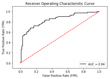
Another metric that's very useful to determine whether your model is well fitted is the Receiver Operating Characteristic (ROC) curve. The metrics module has the roc_curve() function that helps you to generate a ROC curve, as well as the auc() function that calculates the area under the ROC curve.
The following code snippet plots the ROC curve and displays the AUC (Area Under Curve) (see Figure 7):
from sklearn.metrics import roc_curve, auc
import matplotlib.pyplot as plt

# convert the probabilities from ndarray to
# dataframe
df_prob = pd.DataFrame(pred_probs, columns=['Death', 'Survived'])

fpr, tpr, thresholds = roc_curve(test_label, df_prob['Survived'])

# find the area under the curve (auc) for the ROC
roc_auc = auc(fpr, tpr)

plt.title('Receiver Operating Characteristic Curve')
plt.plot(fpr, tpr, 'black', label='AUC = %0.2f'% roc_auc)

plt.legend(loc='lower right')
plt.plot([0,1],[0,1],'r--')
plt.xlim([-0.1,1.1])
plt.ylim([-0.1,1.1])

plt.ylabel('True Positive Rate (TPR)')
plt.xlabel('False Positive Rate (FPR)')
plt.show()

print(fpr) # Increasing false positive rates such
           # that element i is the false positive
           # rate of predictions with score >= thresholds[i].
print(tpr) # Increasing true positive rates such
           # that element i is the true positive
           # rate of predictions with score >= thresholds[i].

print(thresholds)
For the R programmer, I've listed the solution for the Titanic problem written in R, as shown in Listing 3.
Listing 3: Logistic Regression using R for the Titanic Dataset
# load the titanic training set
training.data.raw <- read.csv('Titanic_train.csv', header = T, na.strings = c(""))
print(head(training.data.raw))

#-----------------------------------------------------------------#

# print number of rows
print (c("Number of rows: ", nrow(training.data.raw)))

#-----------------------------------------------------------------#

# examine which are the columns with NA values
sapply(training.data.raw, function(x) sum(is.na(x)))

    # the sapply() function applies the function
    # passed as argument to each column of the dataframe

#-----------------------------------------------------------------#

# get the number of unique values for each column
sapply(training.data.raw, function(x) length(unique(x)))

#-----------------------------------------------------------------#

# we are only interested in the following features -
# Survived (2), Pclass(3), Sex(5), Age(6), SibSp(7),
# Parch(8), Fare(10), Embarked(12)
data <- subset(training.data.raw, select = c(2,3,5,6,7,8,10,12))
print(head(data))

#-----------------------------------------------------------------#

# omit the rows with empty values
data <- na.omit(data)

# OR, fill the empty values for age with the average age
# data$Age[is.na(data$Age)] <- mean(data$Age, na.rm=T)
# na.rm=T means NA values should be stripped before computation

print(data)

#-----------------------------------------------------------------#

# remove all rows with Embarked empty
data <- data[!is.na(data$Embarked),]

# check if there are NaN in data
sapply (data, function(x) sum(is.na(x)))

# check the length of unique values for each column
sapply(data, function(x) length(unique(x)))

#-----------------------------------------------------------------#

# check if Sex, Pclass, and Embarked are categorical values
is.factor(data$Sex)      # read.csv() by default will
                         # encode the string variables as factors
is.factor(data$Embarked) # read.csv() by default will encode the
                         # string variables as factors
is.factor(data$Pclass)
is.factor(data$Survived)

#-----------------------------------------------------------------#

data$Pclass <- factor(data$Pclass)      # make Pclass a catagorical value
data$Survived <- factor(data$Survived)  # make Survied a categorical value

is.factor(data$Pclass)
is.factor(data$Survived)

print(head(data))

#-----------------------------------------------------------------#

# get the number of rows in data
n <- nrow(data)

data.shuffled <- data[sample(n), ]          # shuffle the data
print(head(data.shuffled))

train.indices <- 1:round(0.75 * n)          # indices for the first 75% of the rows
train <- data.shuffled[train.indices,]      # get the first 75% of the rows

train.indices <- (round(0.75 * n) + 1):n    # indices for the remaining 25% of the rows
test <- data.shuffled[train.indices, ]      # get the remaining 25% of the rows

print(nrow(train))
print(nrow(test))

#-----------------------------------------------------------------#

# create a glm() instance - Generalized Linear Models
model <- glm(Survived ~ .,                       # Survived is the label and
             family=binomial(link='logit'),      # features are the rest of
             data=train)                         # the data column
summary(model)

#-----------------------------------------------------------------#

# make predictions
pred.results <- predict(model,  # don't pass in the Survived (1) column
                        newdata=subset(
                           test,
                           select=c(2,3,4,5,6,7,8)),
                        type='response')

pred.results <- ifelse(pred.results > 0.5,1,0)  # if value>0.5
                                                # assign 1 else 0
print(pred.results)

#-----------------------------------------------------------------#

# find all the ones where prediction
# is correct and calculate the mean
accuracy <- mean(pred.results == test$Survived)
print(paste('Accuracy',accuracy))

#-----------------------------------------------------------------#

# installing the ROCR package
# run this only once
# install.packages('ROCR', repos='http://cran.us.r-project.org')
library(ROCR)

# make predictions
p <- predict(model, newdata = subset(test,select=c(2,3,4,5,6,7,8)), type="response")
print(p)

# transform the input data into a standardized format
# needed by ROCR
pr <- prediction(p, test$Survived)

# perform all kinds of predictor evaluations
prf <- performance(pr, measure = "tpr", x.measure = "fpr")
plot(prf)

auc <- performance(pr, measure = "auc")
auc <- auc@y.values[[1]]
auc

#-----------------------------------------------------------------#

# installing the caret package
# run this only once
install.packages('caret', dependencies = TRUE)
library(caret)

p <- ifelse(p > 0.5,1,0)

# print the confusion matrix
confusionMatrix(p, test$Survived)
Summary
In this article, you've learned how to implement machine learning using Python and the Scikit-learn library. In particular, you've used the LinearRegression and LogisticRegression classes to solve regression and classification problems, respectively. In addition, the solution for the Titanic problem is also presented in R.


