In my previous article (Nov/Dec 2017 CODE Magazine), I talked about machine learning using Python and the Scikit-learn library. In addition to using Python for data science and machine learning, another language is very popular among data scientist and statisticians, and that's R. R is an open-source programming language and software environment for statistical computing and graphics. R is based on another language, S, created by John Chambers while he was at Bell Labs. The name R was partly due to the names of its two creators, Ross Ihaka and Robert Gentleman at the University of Auckland, New Zealand. It was also partly because it was seen as a dialect of the S language.
Regardless of the history behind its name, R and its libraries implement a wide variety of statistical techniques, such as linear and nonlinear modeling, classical statistical tests, time-series analysis, classification, clustering, and others. Another core strength of R is graphics, which can produce publication-quality graphs. All of these qualities make R a dream language for statisticians and data scientists.
In this article, I'll start out with an introduction to the R language so that you can get up to speed quickly. In the next article, I'll dive into the various libraries in R that you use for machine learning.
Trying Out R
To try out R, you have a number of options. First, if you followed my previous article on using Python with Scikit-learn, you installed Anaconda (https://www.anaconda.com/download). (If you didn't already do this, please follow the “Installing Anaconda” sidebar's link.) Although the Anaconda installation only comes with Python support by default, you could easily add R support in Anaconda (https://conda.io/docs/user-guide/tasks/use-r-with-conda.html) by running a simple command in Terminal. To install R in Anaconda, type the following command in Terminal and follow the on-screen instructions:
$ conda install r-essentials
The above command installs the libraries for R in your Anaconda installation. Once this is done, you can launch Jupyter Notebook. Doing so brings up the development environment using your Web browser:
$ jupyter notebook
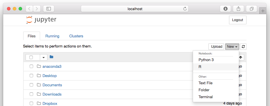
The above command launches the Web browser. To start an R session, click New > R (see Figure 1).
You should now see the familiar notebook, as shown in Figure 2.

Another popular editor for running R code is RStudio (https://www.rstudio.com). I'll be using Jupyter for this article.
Basic Language Syntax
R is a dynamically typed language, meaning that variables need not be pre-declared with a specific data type. Rather, variables take on whatever type is necessary, based on the value assigned to them. The following statements show some examples:
num1 <- 5.5
6 -> num2
print(num1)  # 5.5
print(num2)  # 6

num2 = "Two"
print(num2)  # "Two"
In R, the assignment operator is <- or -> (although the usual = operator is also supported).
To check the data type of variables, use the typeof() function:
print(typeof(num1))  # "double"
print(typeof(num2))  # "character"
You can also perform multiple assignments in a single statement, like this:
num2 = 6
num4 <- num3 <- num2
print(num3)                  # 6
print(num4)                  # 6
One common misconception when dealing with string variables is to assume that the length() function returns the length of the string, as the following example illustrates:
str = "This is a string"
print(str)           # "This is a string"
print(length(str))   # 1
Interestingly, the length() function returns a 1 for the above example. This is because the length() function returns the length of vectors (the section on Vectors later in this article covers this more fully). In R, every variable is also of the type vector. Think of a vector as an array in a typical conventional programming language. So, in the above example, length(str) actually returns the number of items in the str vector, which is 1. To get the length of a string variable, use the nchar() function, like this:
print(nchar(str)) # 16
Using Functions in R
In R, you can get more information about a specific function by using the print() function. For example:
print(exp)
# function (x)  .Primitive("exp")
The above code statement shows the exp() function, which takes in a single argument and returns a primitive result. Here's another example:
print(log)
# function (x, base = exp(1))  .Primitive("log")
The log() function takes in two arguments. The second argument has a default value of exp(1) and the function returns a primitive result.
You can now see how to call the log() function using the various combinations of arguments:
print(log(10))                # 2.302585
print(log(10, base=exp(1)))   # 2.302585
print(log(10, base=10))       # 1
print(log(10, 10))            # 1
print(log(base=exp(1), x=10)) # 2.302585
print(log(base=exp(1), 10))   # 2.302585
Note that you can swap the order of the arguments if you specify the argument names. This is very useful as it makes the function calls much more self-explanatory. They are also some scientific and mathematical functions in R:
print(sin(90))                # 0.8939967
print(cos(180))               # -0.5984601
print(tan(270))               # -0.1788391

print(factorial(6))           # 720

print(round(3.14))            # 3
print(round(3.145, 2))        # 3.15
Defining Your Own Functions
To define your own function, you can use the function keyword and then assign it to a function name, like the following:
myFunction <- function(n,m = 6) {
    result = n * m
    result + 5         # OR return (result + 5)
}
In the above example, myFunction takes two arguments: n and m. The parameter m is known as the default parameter, which has a default value of 6 when you don't supply it when calling the function. Note that the last statement in a function is used as the return value, so essentially the return keyword is optional. I prefer to use the return keyword, as this makes the function clearer. The following statements show how to call the function, the first with one argument and the second with two arguments:
print(myFunction(5))    # 35
print(myFunction(5,7))  # 40
Making Decisions
To make decisions, R uses the familiar if-else statement construct. The following shows an example of a function that determines if a number is an odd number:
isodd <- function(n) {
    if (n %% 2 == 0) {    # %% is modulus
        FALSE
    } else {
        TRUE
    }
}

isodd(46)    # FALSE
isodd(45)    # TRUE
If you're one who indulges in terse coding, the above isodd() function can be rewritten as a single statement:
isodd <- function(n) {(n %% 2 != 0)}
R supports the usual arithmetic, relational, and logical operators:
- + (addition), - (subtraction), * (multiplication), / (division), ^ (power), %% (modulo)
- > (greater than), < (lesser than), == (equality), <= (lesser or equal to), >= (greater than or equal to), != (not equal to)
- && (logical AND), || (logical OR), ! (logical NOT)
Vectors
As briefly mentioned earlier, everything in R is a vector. Think of a vector as an array of items of the same data type.
x <- c(3,4,5,6,7)
print(typeof(x))      # double
print(length(x))      # 5
In that snippet, x is a vector comprised of five items of type double. You can append additional items into the vector using the c() function:
x <- c(x, 8)          # append another item to x
print(x)              #  3 4 5 6 7 8
If you append an item of a different type to the existing vector, R attempts to convert all items in the vector into a common type, as the following example shows:
x <- c(x, "9")        # append another item to x
print (x)             #  "3" "4" "5" "6" "7" "8"
                      #  "9"
x <- c(x, TRUE)
print(x)              #  "3"    "4"    "5"
                      #  "6"    "7"    "8"
                      #  "9"    "TRUE"
If you want to have a collection of items with different types, use a list instead of a vector, like this:
y <- list(3,4,5,6,7,"9",TRUE)
Vector Functions
In R, there are a number of vector functions that make manipulating numbers easy. Here's an example:
nums <- c(12,34,56,9,45,67,90,11,2,45)
print(min(nums))     # 2
print(max(nums))     # 90
print(mean(nums))    # 37.1
print(median(nums))  # 39.5
print(sd(nums))      # 28.90002
print(sort(nums))    # 2  9 11 12 34 45 45 56
                     # 67 90
print(sum(nums))     # 371
print(unique(nums))  # 12 34 56  9 45 67 90
                     # 11  2
As you can see, given a vector containing numbers, it's very easy to get information from the vector using the various vector functions such as min(), max(), etc. In particular for data science, you can use the summary() function to get a summary of the numbers contained in the vector:
print(summary(nums))
#    Min. 1st Qu.  Median    Mean 3rd Qu.
#    Max.
#    2.00   11.25   39.50   37.10   53.25
#    90.00
Dealing with NAs
A lot of times, you load data from files, in particular, CSV or tab-separated files. These data files may contain “holes” in them, meaning missing data for some rows and columns. When loading missing values from a CSV file, R automatically replaces them with NAs (for Not Available). One good use of the summary() function is to show the number of NAs in a vector so that you can decide if you need to replace or omit them from the vector before you do any further processing. The following code example shows the summary() function displaying the number of NAs in the vector:
nums <- c(12,34,56,9,45,67,90,11,2,45, NA)
print(summary(nums))
#    Min. 1st Qu.  Median    Mean 3rd Qu.
#    Max.          NA's
#    2.00   11.25   39.50   37.10   53.25
#   90.00   1
To omit the NAs in your vector, use the na.omit() function:
print(sum(na.omit(nums)))  # omit the NAs in
                           # the vector and
                           # sum up the rest
If you want to know whether each element in the vector is a NA, use the is.na() function:
print(is.na(nums))         # FALSE FALSE FALSE
                           # FALSE FALSE FALSE
                           # FALSE FALSE FALSE
                           # FALSE  TRUE
To extract all the numbers in a vector that isn't an NA, use the subset() function:
nums <- subset(nums, is.na(nums) == FALSE)
print(nums)    # 12 34 56  9 45 67 90 11  2 45
Sequencing
When performing data science operations, you often need to generate a sequence of numbers. Instead of creating a vector of numbers manually, it would be easier to be able to generate the sequence automatically. The following code snippet generates a sequence from 1 to 3:
i <- 1:3      # generate a sequence from
# 1 to 3
print(i)      # 1 2 3
You can also generate a sequence in the reverse order:
j <- 5:1
print(j)      # 5 4 3 2 1
You can also use the seq() function to generate a sequence of numbers:
y <- seq(9)
print(y)      # 1 2 3 4 5 6 7 8 9
The seq() function is useful when you want to specify an increment for the sequence, like the following:
y <- seq(from=2, to=9, by=2)
print(y)                # 2 4 6 8
You can also specify the length of the sequence as well as the starting and ending number and the seq() function automatically divides the numbers equally:
y <- seq(from=1, to=1.9, length=20)
print(y)
#  [1] 1.000000 1.047368 1.094737 1.142105
#      1.189474 1.236842 1.284211 1.331579
#  [9] 1.378947 1.426316 1.473684 1.521053
#      1.568421 1.615789 1.663158 1.710526
# [17] 1.757895 1.805263 1.852632 1.900000
If you want to generate a sequence of identical numbers, use the rep() (for repeat) function:
zeros <- rep(0, time=20)
print(zeros)              # 0 0 0 0 0 0 0 0 0 0
                          # 0 0 0 0 0 0 0 0 0 0
The rep() function can also be used to repeat a vector, as the following demonstrates:
cars <- c("Suzuki", "Toyota", "Mercedes")
manycars <- rep(cars, each=2)
print(manycars)
# "Suzuki"   "Suzuki"   "Toyota"   "Toyota"
# "Mercedes" "Mercedes"
Vector Indexing
You can use a sequence as an index into a vector to retrieve the items you want, as the following shows:
x <- c(3,4,5,6,7)
i <- 1:3
print(x[i])             # 3 4 5
To omit an item in a vector, specify the index of the item to omit and prefix it with a negative sign, like this:
print(x[-1])          # 4 5 6 7
# excludes the first item
print(x[-2])          # 3 5 6 7
# excludes the second item
print(x[-length(x)])  # 3 4 5 6
# excludes the last item
To get the last n items from a vector, use the tail() function, like this:
print(tail(x,1))        # 7
print(tail(x,2))        # 6 7
You can also specify a range of items to extract from a vector, like this:
print(x[-2:-3])      # 3 6 7
                     # excludes second through
                     # third items
print(x[1:length(x)-1]) # 3 4 5 6
                     # excludes the last item
You can also specify conditions, like this:
print(x[x > 5])              #  6 7
print(x[x %% 2 == 0])        #  4 6
Looping
R supports looping constructs that are commonly found in other programming languages. The following example shows the for loop in action:
# function to print the first n numbers of the
# fibonacci numbers
fib <- function(n) {
    x <- c(1,1)
    for (i in 2:(n-1)) {
        x <- c(x, sum(tail(x,2)))
    }
    return (x)
}

print(fib(8))      # 1  1  2  3  5  8 13 21
You can also use the while loop in R; in the following example, I used it to create a Fibonacci sequence up to the number specified:
# function to print the fibonacci sequence until
# the n numbers specified
fib <- function(n) {
    x <- c(1,1)
    while (tail(x,1) < n) {
        x <- c(x, sum(tail(x,2)))
    }
    return (x)
}

print(fib(13))               # 1  1  2  3  5  8 13
Data Frames
A lot of times, data is represented in tabular format. This is something that R excels in. Date Frames are extremely useful in data science operations as data is often stored in CSV files or Excel spreadsheets. Loading the data into data frames allows you to manipulate the data using rows and columns.
Creating a Data Frame from Vectors
The following code snippet shows how a data frame (think of it as a table) is created from three vectors:
# column 1
c1 = c(2, 3, 5)

# column 2
c2 = c("aaa", "bbb", "ccc")

# column 3
c3 = c(TRUE, FALSE, TRUE)

# create a data frame using the 3 columns
df = data.frame(c1,c2,c3)

print(df)
Printing the data frame produces the following output:
c1  c2    c3
1  2 aaa  TRUE
2  3 bbb FALSE
3  5 ccc  TRUE
Changing the Column Names of a Data Frame
Note that the column names take on the names of the three vectors by default. You can change this by specifying the column name explicitly:
df = data.frame(col1 = c1, col2 = c2, col3 = c3)
print(df)
The above changes produce the following output with the new column names:
col1 col2 col3
1    2  aaa TRUE
2    3  bbb FALSE
3    5  ccc TRUE
Extracting Columns
To print out a specific column, use the index of the column (remember, index in R starts with 1, not 0):
print(df[2]) # second column
The above prints out this:
col2
1  aaa
2  bbb
3  ccc
You can also print out a column using its column name, like this:
print(df["col3"])
'
col3
1  TRUE
2 FALSE
3  TRUE
'
Note that the preceding prints out a data frame containing only the third column. If you want the values of the third column as a vector, you can use the following syntax:
print(df$col3)  # same as print(df[,"col3"])
'
[1]  TRUE FALSE  TRUE
'
Extracting Rows
To print out a specific row in a data frame, specify its row index:
print(df[2,])
'
col1 col2  col3
2    3  bbb FALSE
'
To print out a specific item in a data frame, specify its index and column number:
print(df[2,3])
'
[1] FALSE
'
Transposing a Data Frame
You can also transpose a data frame using the t() function:
print(t(df))
'
[,1]    [,2]    [,3]
col1 "2"     "3"     "5"
col2 "aaa"   "bbb"   "ccc"
col3 " TRUE" "FALSE" " TRUE"
'
The t() function converts rows to columns and columns to rows.
Subsetting Data Frames
To create a subset of a data frame based on certain criteria, use the subset() function:
true_col = subset(df, col3 == TRUE)
print(true_col)
'
col1 col2 col3
1    2  aaa TRUE
3    5  ccc TRUE
'
The previous snippet retrieves a subset of the df data frame based on the value of the “col3” column. The statements in this next snippet filters the result based on column names:
true_col = subset(df, col3 == TRUE,
select = c(col1, col2))
print(true_col)
'
col1 col2
1    2  aaa
3    5  ccc
'
Creating a Data Frame from Files
For data science work, most of the time you create a data frame directly from a file, such as a CSV, or tab-separated file. Suppose you have the following content saved as a file named fruits.csv:
orange,pineapple,durian
2,3,4
4,5,2
5,3,1
3,2,5
6,8,10
The following code snippet reads the above CSV file into a R data frame and prints it out:
fruits <- read.csv(file = "fruits.csv")
print(fruits)
'
orange pineapple durian
1      2         3      4
2      4         5      2
3      5         3      1
4      3         2      5
5      6         8     10
'
Sometimes the CSV files might not be located locally but resides on a Web server. In this case, you can download it as a file before reading it into a data frame:
download.file(url = "http://bit.ly/2iJjdpb", destfile = "crimerecords.csv")
crimerecords <- read.csv(file = "crimerecords.csv")
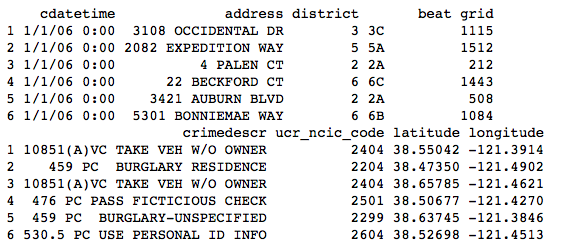
The preceding prints out the output, as shown in Figure 3. The head() function returns the first n rows of the data frame, which by default is the first six rows. Likewise, if you want to print the last n rows of the data frame, use the tail() function.
Plotting Charts Using Data Frame
One of the key features of R is its strong graphic capabilities. Using R, you can directly plot graphs and charts. In the following sections, I'll discuss how to plot some interesting charts in R.
Plotting Bar Charts
Suppose you have a CSV file named public_transport.csv containing the following content:
Gender,Age,Mode,Times
male,25,bus,20
female,28,train,10
male,35,bicycle,20
male,23,bus,7
female,43,bus,24
female,19,train,16
male,41,bus,28
female,12,bicycle,10
male,32,bus,19
female,29,train,19
female,11,bus,7
male,22,train,8
female,26,train,23
female,27,train,31
male,37,train,32
male,31,train,22
That CSV file contains a listing of commuters and their age, their mode of transport and how many times they used the specified mode of transport every month. The following code snippet first loads the CSV file into a data frame:
freq <- read.csv(file = "public_transport.csv")
# count the total occurences of each "Mode" of transportation
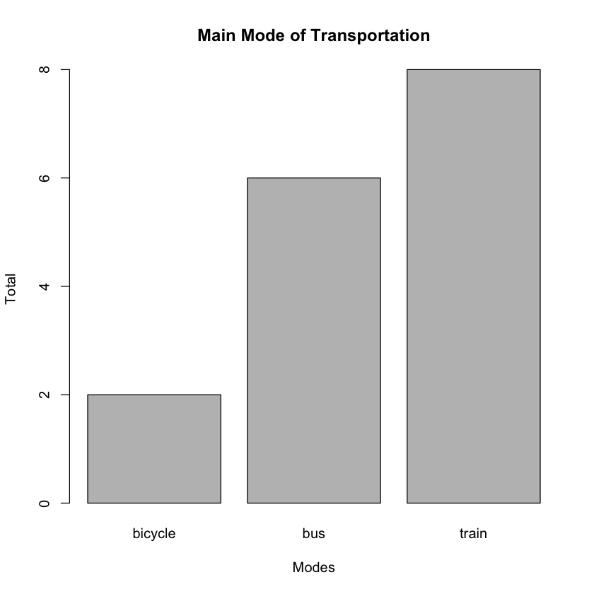
Suppose you want to know the number of people using bicycles, buses, and trains. To do this, you can use the table() function, which will help you tabulate the frequencies of each occurrence of transport mode:
freqMode <- table(freq$Mode)
print(freqMode)
'
bicycle     bus   train
      2       6       8
'
Using the result returned by the table() function, you can plot a bar chart using the barplot() function:
barplot(freqMode,
    main="Main Mode of Transportation",
    xlab="Modes",
    ylab="Total")
The main argument specifies the title of the chart, while the xlab and ylab arguments specify the x-axis and y-axis labels respectively. The bar chart created is shown in Figure 4.
You can also alter the density of the bars by specifying the density argument:
barplot(freqMode,
    main="Main Mode of Transportation",
    xlab="Modes",
    ylab="Total",
    border="blue",
    density=c(10,20,30,40,50))
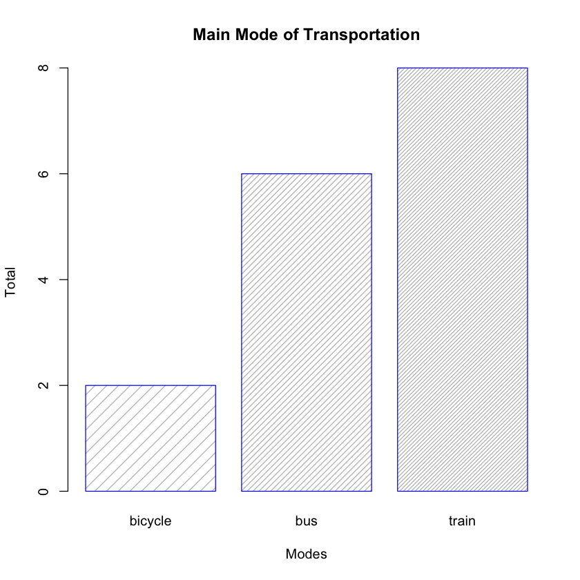
The density argument is a vector giving the density of shading lines, in lines per inch, for the bars or bar components. The bar chart now looks like Figure 5.
Besides loading a data frame from a CSV file, you can also load it from a tab-separated file, such as the following example of a file named fruits.txt that contains the sales of the various fruits for each month from January to May:
orange pineapple    durian
     2         3         4
     4         5         2
     5         3         1
     3         2         5
     6         8        10
The following code snippet loads the content of the file into a data frame:
fruits_data <- read.table("fruits.txt", header=T, sep="\t")
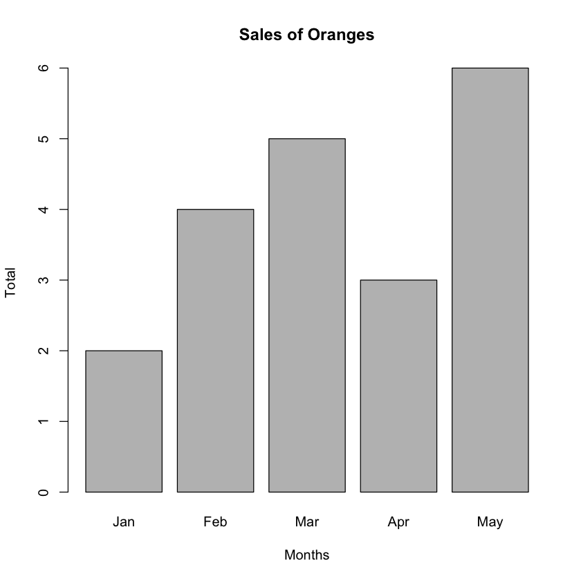
Next, plot a bar chart showing the sales of oranges for each of the five months:
barplot(fruits_data$orange,
    main="Sales of Oranges",
    xlab="Months",
    ylab="Total",
    names.arg=c("Jan","Feb","Mar","Apr","May"))
The names.arg argument is a vector of names to be plotted below each bar or group of bars. The bar chart is shown in Figure 6.
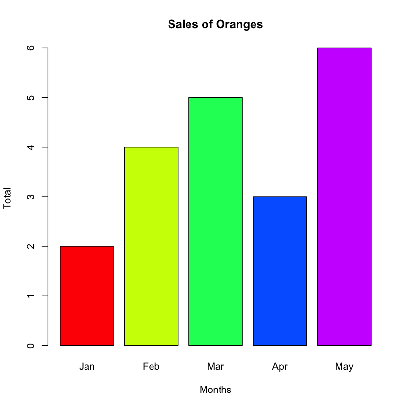
You can change the colors of the bars (see Figure 7) by using the col argument:
fruits_data <- read.table("fruits.txt", header=T, sep="\t")

barplot(fruits_data$orange,
        main="Sales of Oranges",
        xlab="Months",
        ylab="Total",
        names.arg=c("Jan","Feb","Mar","Apr","May"),
        col=rainbow(5))
The col argument is a vector of colors for the bars or bar components. You can use the rainbow() function to generate a set of colors. For example, the rainbow(5) statements generates a vector containing the following five elements: “#FF0000FF”, “#CCFF00FF”, “#00FF66FF”, “#0066FFFF”, and “#CC00FFFF”.
What about displaying the sales of the various fruits for each month? You can first convert the data frame into a matrix using the as.matrix() function:
print(as.matrix(fruits_data))
'
     orange pineapple durian
[1,]      2         3      4
[2,]      4         5      2
[3,]      5         3      1
[4,]      3         2      5
[5,]      6         8     10
'
And then plot the bar chart using the matrix:
fruits_data <- read.table("fruits.txt", header=T, sep="\t")
barplot(as.matrix(fruits_data),
    main="Sales of Fruits from Jan to May",
    xlab="Months",
    ylab="Total",
    beside=TRUE,
    col=rainbow(5))
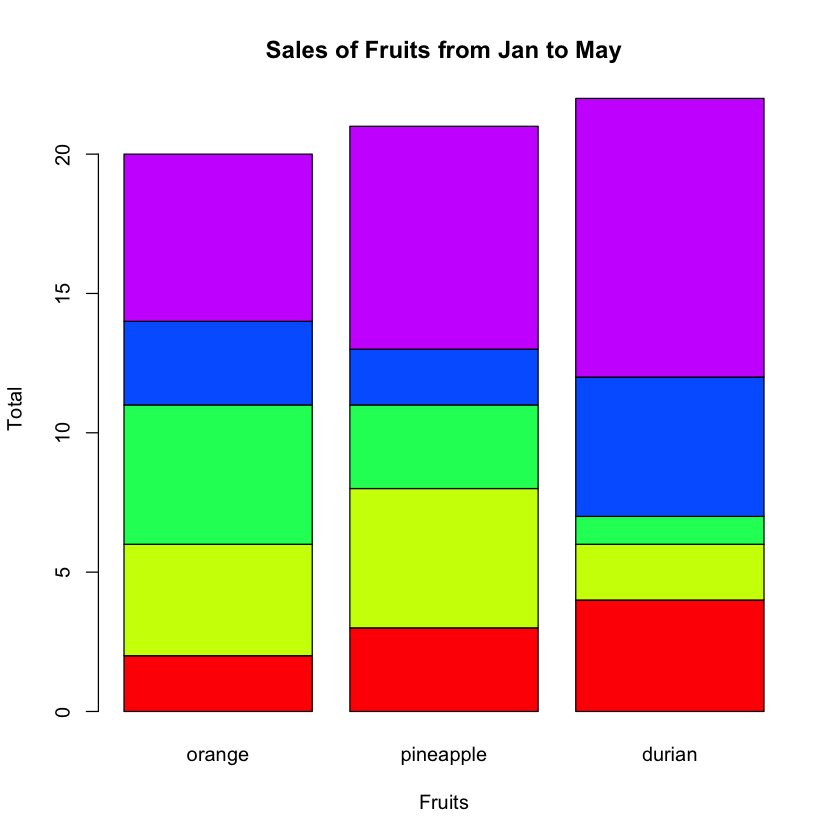
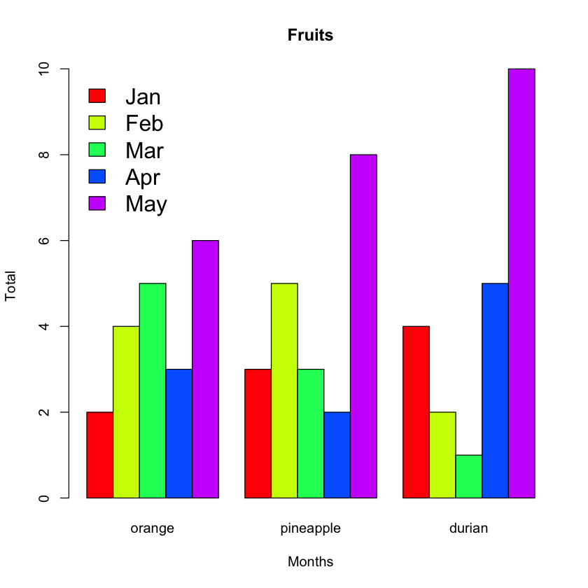
The beside argument specifies whether the columns of height are portrayed as stacked bars (FALSE), or the columns are portrayed as juxtaposed bars (TRUE). Figure 8 shows the bar chart with the beside argument set to TRUE.
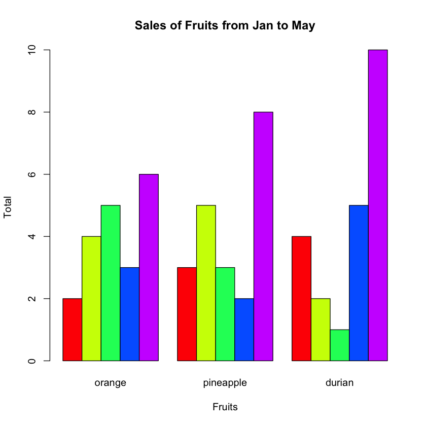
Figure 9 shows the bar chart with the beside argument set to FALSE.
You can display a legend on your chart using the legend() function:
fruits_data <- read.table("fruits.txt", header=T, sep="\t")
barplot(as.matrix(fruits_data),
    main="Sales of Fruits from Jan to May",
    xlab="Fruits",
    ylab="Total",
    beside=TRUE,
    col=rainbow(5))

legend("topleft",
    c("Jan","Feb","Mar","Apr","May"),
    cex=1.6,
    bty="n",
    fill=rainbow(5));
The cex argument specifies the size of the text to be used for the legend. The bty argument takes either “n” or “o”. Setting to “o” draws a rectangle around the legend and setting it to “n” means no rectangle is drawn.
Figure 10 shows the chart with the legend.
Plotting Histograms
A histogram is another type of chart that's very useful for showing the distribution of numerical data. Using the transportation CSV file that I discussed earlier, you can plot the distribution of the commuters' age using a histogram, as shown in the following code snippet:
freq <- read.csv(file = "public_transport.csv")
histogram = hist(freq$Age,
    main ="Distribution of Age groups",
    xlab = "Age Range",
    ylab = "Total")
Figure 11 shows the histogram showing the distribution of the ages of the commuters.

Observe that R automatically breaks the data up into intervals. You can verify this by printing the breaks property:
print(histogram$breaks)
'
[1] 10 15 20 25 30 35 40 45
'
Sometimes you want to have more control over the breaks, and you can indeed do so via using the breaks argument by passing it a sequence, like this:
histogram = hist(freq$Age,
main ="Distribution of Age groups",
xlab = "Age Range",
ylab = "Total",
breaks = seq(0,50, by=10))
The updated histogram looks like Figure 12.

Plotting Scatter Plots
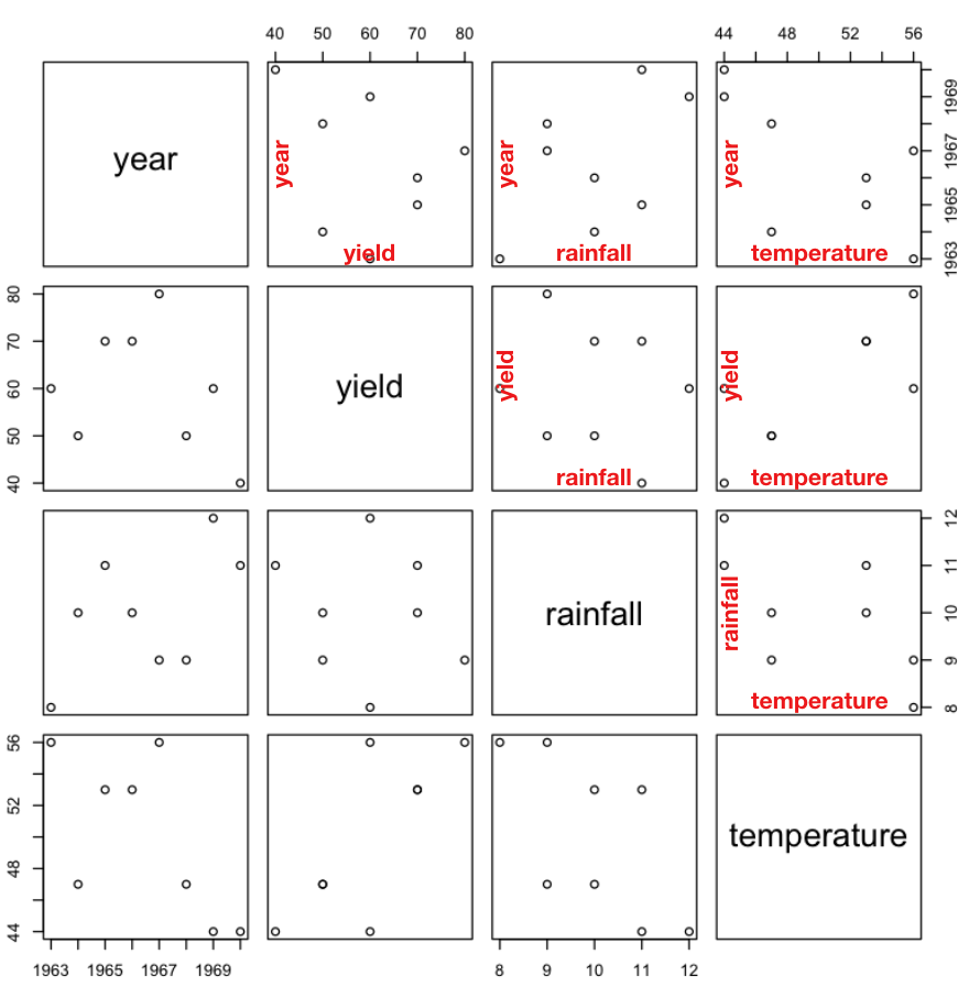
Scatter plots are useful for plotting data points on a horizontal and a vertical axis when attempting to show how much one variable is affected by another. Consider the following example CSV file, named rainfall.csv, containing the yield of a particular crop and the associated rainfall and average temperature for a particular year.
year,yield,rainfall,temperature
1963,60,8,56
1964,50,10,47
1965,70,11,53
1966,70,10,53
1967,80,9,56
1968,50,9,47
1969,60,12,44
1970,40,11,44
You could plot a scatter plot using the plot() function:
rainfall <- read.csv(file = "rainfall.csv")
plot(rainfall[1:4])
Figure 13 shows the scatter plot.

Using the scatter plot, you can compare the relationships among the various factors, such as year, yield, rainfall, and temperature. Figure 14 shows how to read the scatter plot.
Plotting Pie Charts
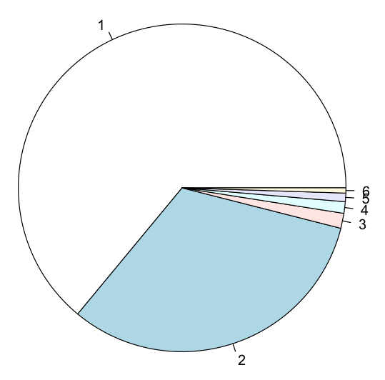
A pie chart displays a circle divided into slices to illustrate numerical proportion. In R, you can display a pie chart using the pie() function. Consider the following code snippet, which has a vector containing the market share of operating systems:
os <- c(63.99, 32.03, 1.48, 1.14, 0.84, 0.51)
pie(os)
The pie chart created is shown in Figure 15.
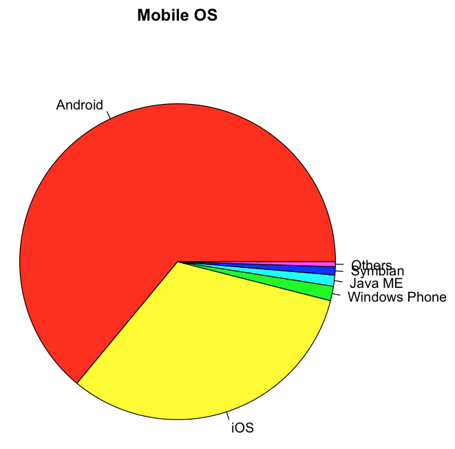
You could supply additional information to make the pie chart more descriptive by adding labels:
pie(os,
    main="Mobile OS",
    col=rainbow(length(os)),
    labels=c("Android","iOS","Windows Phone",
             "Java ME","Symbian", "Others"))
Figure 16 shows the pie chart that is color-coded, with labels representing each slice of the pie.
As you saw earlier, you can generate a vector of color using the rainbow() function. In addition to this function, you can use the various other color palettes in R:
- heat.colors(n)
- terrain.colors(n)
- topo.colors(n)
- cm.colors(n)
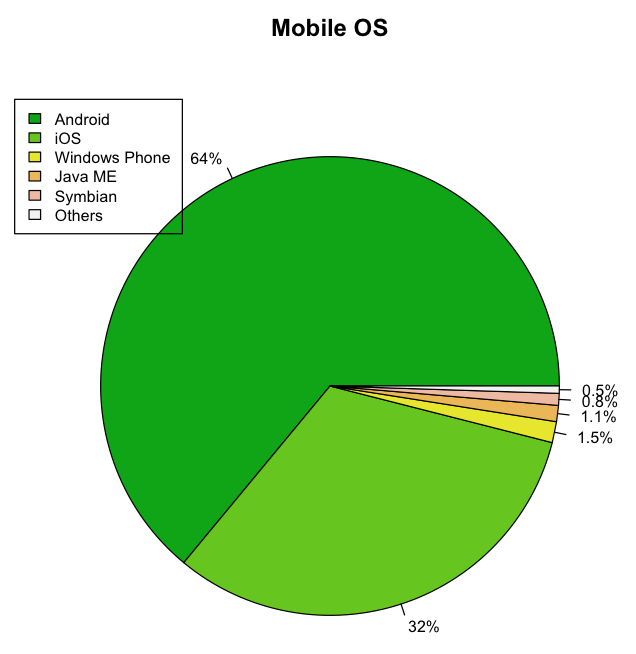
The following code snippet shows a more detailed pie chart (see Figure 17) displaying the percentage of each slice as well as displaying a legend:
colors <- terrain.colors(6)

# calculate the percentage
os_labels <- round(os/sum(os) * 100, 1)

# concat a % after each value
os_labels <- paste(os_labels, "%", sep="")

pie(os,
    main="Mobile OS",
    col=colors,
    labels=os_labels, cex=0.8)

legend(-1.1,
    1,
    c("Android","iOS","Windows Phone",
    "Java ME","Symbian", "Others"),
    cex=0.8,
    fill=colors)
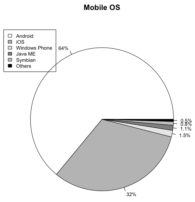
Besides the palette of colors, you can also create your own sets of grey tones:
colors <- c("white","grey70","grey90",
"grey50","grey75","black")
Figure 18 shows the pie chart using different shades of grey.
Summary
In this article, you had a whirlwind tour of R. Although this isn't an attempt to teach you everything about R, I do believe getting acquainted with the language can make you ready to embrace machine learning. In addition to the language basics, you also learned how to visualize data by using the various functions in R to plot charts, such as pie charts, bar charts, histograms, and scatterplots.


